Determining the Optimal Level of Inventory
Determining the Optimal Level of Inventory
In this attempt to prevent cost of stock outs and to minimize cost of carrying inventories skilful finance manager aims towards a policy of holding the appropriate level of inventory necessitates the resolution of the conflicting goals. As observed earlier, a larger inventory ensures uninterrupted production and minimizes costs of production interruptions caused by inadequate inventories and risk of loss of profits owing to loss of sales and possible purchase discounts and so on but it accompanies higher carrying costs and the risk of obsolescence. but increases cost of production due to frequent production interruptions and also cost of being of stock. Determination of the right amount of inventory calls for matching of gains derived from carrying additional inventory with the costs involved in carrying such amount of inventory.
It must also be remembered in this regard that as order increase in size, additional savings decline per unit of added purchase because saving due to fixed cost is spread over a larger number of units even if quantity discounts are availed of whereas the additional variable costs tend to move up constantly with an increase in size of orders. Therefore, the carrying costs of inventory but the same may not hold true in respect of savings from purchasing or producing inventory and for that matter to balances costs of carrying inventor, the finance manager must consider a number of different levels of inventory for a particular item, and select that level which yields the lowest total cost.
One of the most widely used a technique which provides a fool solution to the problem of determining optimal size of inventory in a firm is Economic Order Quantity’ (EOQ). We shall now discuss as to how optimal size of inventory is determined under EOQ approach.
According to EOQ approach, optimal level of investment in inventory is one where total costs of inventory comprising carrying and acquisition costs will be the minimum. This is also known as economic order quantity. The approach begins with analysis of behavioural relationship between carrying cost and acquisition cost and total cost at different levels of ordering inventories. Thus, the cost of carrying raw materials inventories costs of ordering inventories cost of placing orders, quantity discounts lost and so on declines with an increase in size of inventory. The net effect of these rises and falls on total costs will depend on magnitude of the changes in those related costs.
The optimum quantity of ordering can be found by the following equation:
EOQ = √2KD/P|1
Where
D = Annual usage rate
P = Unit purchase price of inventory item
I = Annual inventory carrying charge as a percent of inventory value.
K = Acquisition cost per order.
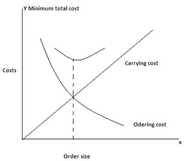
Another method of determining the economic order quantity is graphic method. Figure 1 demonstrates the results of plotting the total inventory costs for various order quantities. The acquisition costs which tend to decline with an increase in quantum. of order are designed by curve ‘D’. Carrying costs which rise constantly are represented by curve ‘R’. Curve ‘T’ represent total inventory costs. The point where curves D and R interest cash other is the lowest inventory cost per order.
The EOQ model of inventory management is a very useful technique of controlling inventories. Thus, it tells us how much quantity of raw materials the firm should order to ensure uninterrupted production at minimum cost. It also enables the firm to exercise suitable control over. The size of production runs.