Geometric Analysis
The concept of increasing and decreasing functions, so also, that of the maxima and minima will be clearer from the geometric analysis made as under:
Let the graph of a function f(x) appear as under:
From the above graph, it must be noticed that f(x) is represented by a curve in a plane, and (a, b) is any point on the curve where, b = f (a).
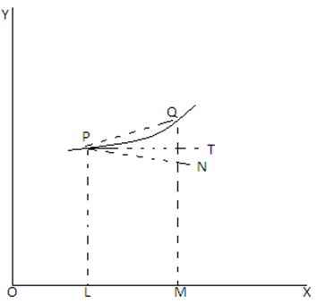
Let p and Q be the two points on the curve. If P be (x,y), then Q can be taken as (x + x, y + y). If x and y are very small, then P and Q will be the points on the curve close to each other.
Let us draw PL and QM as perpendiculars to the base, and PN as perpendicular to MQ.
Now, PN = LM = OM – OL
= (x +x ) –x = δx
Again, QN = QM – NM = (y + δy) – Y = δy
At this moment, imagine that P is fixed and Q comes closer to P as the line through P and Q is rotating about P. As Q comes closer to P, δx becomes smaller. Finally, when Q coincides with P, the line through P and Q takes the position of the tangent, PT and touches the curve at P. As δx → 0, Q → P and the line PQ → PT.
Now, the ration QN/PN = δy/δx = dy/dx as δx → 0. But δy/δx is the slope of the straight line PQ. The straight line PQ becomes the tangent PT, when δx i.e., the change in X is zero and for which dy/dx will be slope of PT.
If, we carefully observe the variation in the slope depending upon the position of the line, the following important conclusions would be drawn:
(i) If the line is inclined to the right, the slope is positive.
(ii) If the line is inclined to the left, the slope is negative.
(iii) If the line is parallel to the base, the slope is zero.
The zero slope concepts help us in the determination of the maximum and minimum values of a continuous function.